Table of Contents
1. Introduction
An auto dealership often purchases a used car at an auto auction. This used car might have serious issues that cannot sell to customers. The auto community calls these unfortunate purchases “kicks.” The purpose of this project is to build a model to predict if the car purchased at the Auction is a Kick (bad buy). All project data come from the Kaggle. I propose to use logistic regression as the main algorithm to create the classifier. After training and tuning hyperparameter of the classifier, the area under the curve (AUC) of my classifier is 0.73. The F1 score of my classifier is 0.36. The accuracy of the prediction on the testing dataset is 96%. I also provide a well-documented IPython file on Github to explain how to step-by-step analyze this project.
In this project, I will follow steps from Hands-On Machine Learning with Scikit-Learn and TensorFlow. This book provides an excellent strategy how to do an end-to-end machine learning project. I highly recommend this strategy for the machine learning project. I summary general processes for a machine learning project in this report, the process can split into seven steps: understand the problem, get the data, data exploration, data preprocessing, model training, and model tuning and evaluations.
2. Understand the Problem
The project target is to predict if the car purchased at the Auction is a Kick (bad buy).Therefore, I frame this project as a supervised classification problem. Furthermore, this project is a binary classification problem because it predicts help a dealership to identify the purchases is a bad buy or a good buy.
For the binary classification problem, there are three standard methods to evaluate the performance of the model. First, I evaluate the performance of a classifier using F1 score, because the F1 score is the combination of precision and recall, which is the harmonic mean of precision and recall. Also, I evaluate the performance of classifier use AUC of receiver operating characteristic (ROC) curve, because the ROC curve is another common tool used with binary classifiers. Finally, I evaluate the prediction accuracy of the testing dataset.
To sum up, after framing the problem (make an assumption) and select methods to evaluate the model, I can start to get data and to look data information.
3. Get the data
All data come from Kaggle, I download data and use Pandas to load data. However, before directly using Pandas, I write a small class with some loading function to load data (the codes are in IPython file).
Before splitting data into the training and test datasets, I need understand what exactly the data it is. First, I check original data and see the header of data in figure 1.
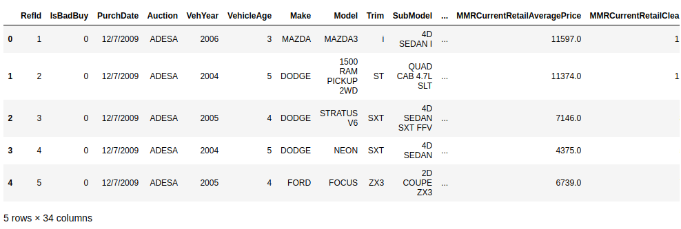
shows the top 5 rows and header of the data.
Here, we can see some feature of data, but it is not enough. Next, I want to know more data details in figure 2 such as total rows of data, numbers of features of data, the type of each feature of data.
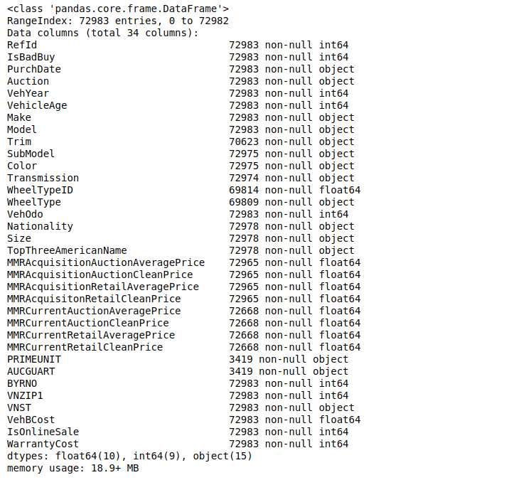
shows details information about this data.
From the output, I can see this data has total 34 features, 72983 rows of data, 19 numeric data, and 16 text data. Then, in figure 3, I know each text data feature, and majority label is “true” for the data.
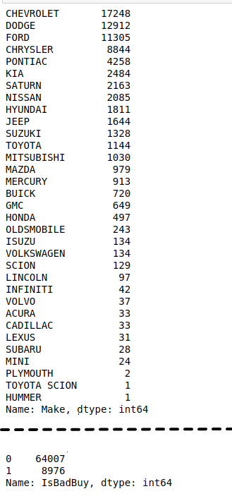
shows each column's data distribution.
In figure 4, I want to know more statistical attributes like the mean of each numeric data or the standard deviation of each numeric data.
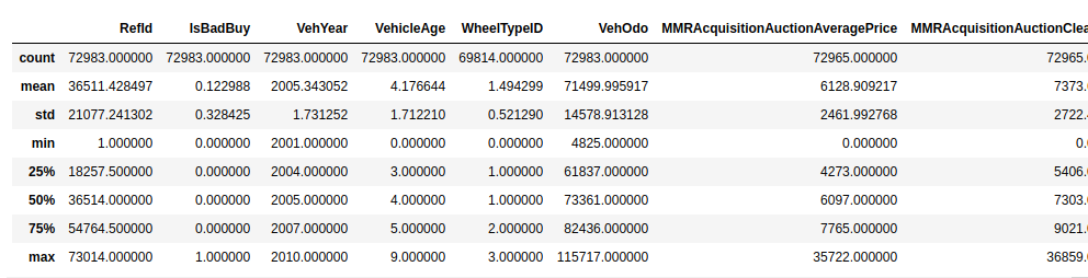
shows each column’s data statistical attributes.
Sometimes, people may prefer to visualize the data distribution, for example, in figure 5. Now I write a class to plot data and save graphs into the target location. The MatPlotlib already have the plot function, but it is a good habit to write a function to combination plot and label, which can reuse later.
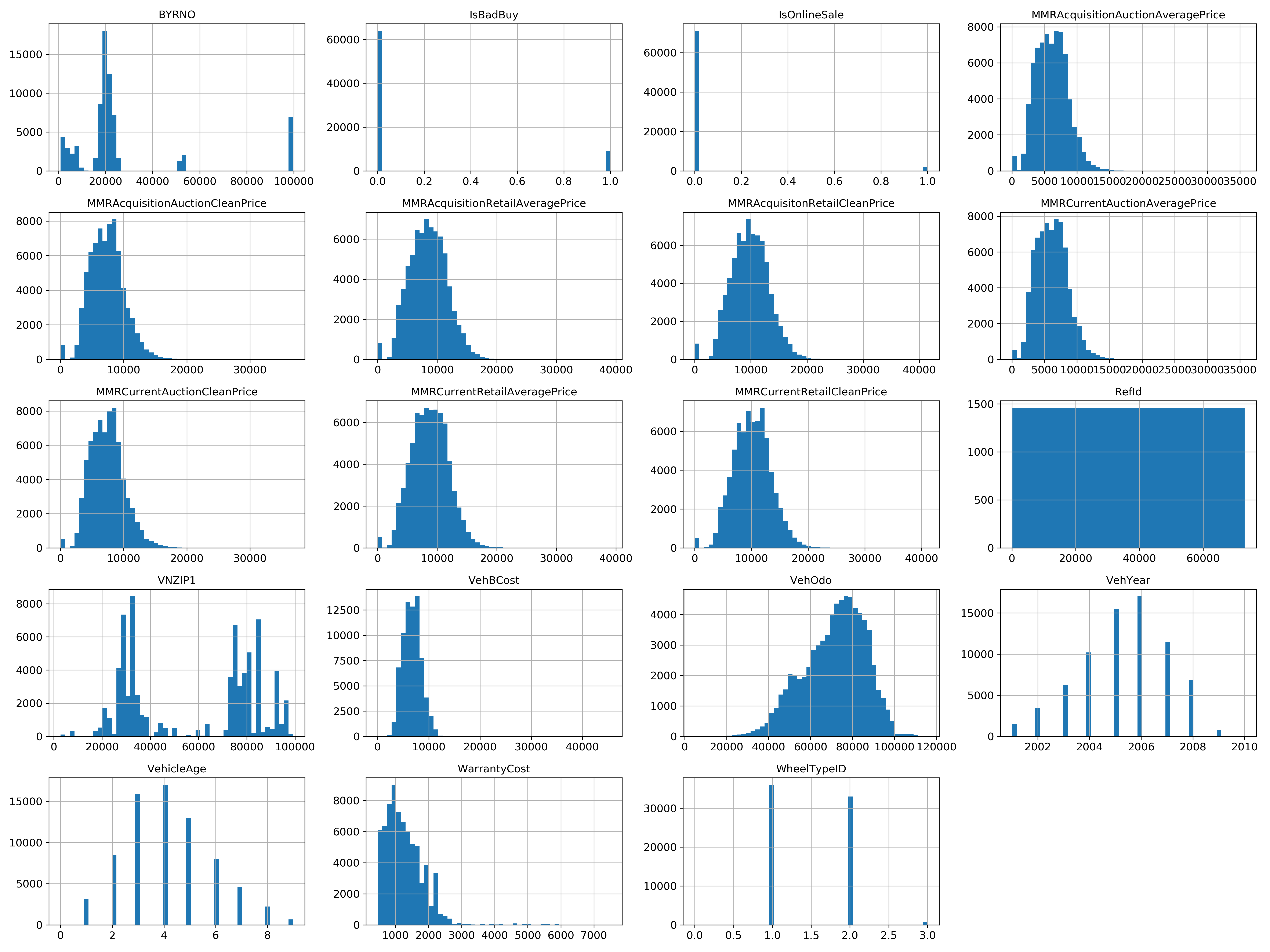
provides diagrams to display data distribution of all numeric columns.
From the “IsBadBuy” diagram, I can also see the majority label is “true,” which is good for us making classification on the test dataset. Also, I see the “VehYear” and “VehicleAge” diagrams have the normal distribution, which means that I can use those two features as the critical features to make a model (have more eigenvalue to make more accuracy model).
To summary, after I understand much information about the data, I can split the data into training and test dataset. However, I need not split datasets because Kaggle already provides training (60%) and test (40%) dataset. If the data need to split, the Scikit-Learn provide a few functions to split datasets into multiple subsets in various ways.)
4. Data Exploration
So far I have only taken a quick glance at the data to get a general understanding of the kind of data I am manipulating. Now, I need to go deep to check more about data. First, I need put the test dataset aside. Since the training dataset is not too large, I can efficiently compute the standard correlation coefficient (also called Pearson’s r) between every pair of attributes, in Figure 6.
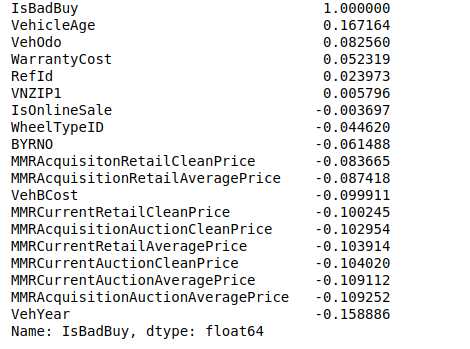
shows standard correlation coefficient.
From the correlation, I see the “VehYear” and “VehicleAge” is the strongest relation with “IsBadBuy.”
One last thing I want to do before actually preparing the data for machine learning algorithms is to try out various attribute combinations. In my opinion, the more miles per year driver drive; the more likely driver will more cause a kick car. Thus, I can create new attribute “miles per year,” and I recheck the standard correlation coefficient in figure 7.
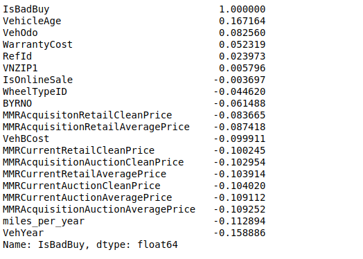
shows standard correlation coefficient after adding a custom attribute.
Now, it’s time to prepare the data for my machine learning algorithms.
5. Data Preprocessing
The best way to prepare data is to use Scikit-Learn’s Pipeline to do it. However, before I create the full pipeline, I need figure out how to create transformer for each part. It includes five steps: data cleaning, handing test and categorical attributes, custom transformer, feature scaling, and transformation pipelines.
Data cleaning
Many times, I noticed that some attributes have some missing values. I can accomplish these efficiently using Pandas’ DataFrame to drop miss data. However, I believed that it would be a waste. I decided to implement the following rules: if the feature includes a continuous value, I will replace the missing value with the average of the feature over the other samples, and if the feature includes a discrete value, I will create a new value specifically to identify missing data. Here, Scikit-Learn provides a handy class to take care of missing values: Imputer.
Handing test and categorical attributes
Earlier I left out many categorical attributes because those are a text attribute so I cannot compute its median. Most machine learning algorithms prefer to work with numbers, so let’s convert these text labels to numbers. The author of Hands-On Machine Learning with Scikit-Learn and TensorFlow provides a method to encoder these text labels. I can use this method to get one-hot encoding easily.
Custom transformer
In previous, I need to add the custom attribute to the training dataset. Therefore, I want to create a custom transformer class to add this step to the pipeline.
Feature scaling
Machine learning algorithms do not perform well when the numerical input attributes have very different scales. Therefore, I can use Scikit-Learn’s StandarScaler for standardization.
Transformation pipelines
Finally, many data transformation steps need to execute in the right order. I can now create a full pipeline to prepare use Scikit-Learn’s Pipeline.
6. Model Training
Since our data is ready, I will start training models now. I will use three algorithms: Logistic Regression, Radom Forests, and Nonlinear SVM. First, I train model use Logistic Regression without tuning it. Moreover, I use 5-fold cross-validation to get the evaluation. For Logistics Regression classifier without tuning, the F1 score is 0.37 and AUC is 0.72. The ROC curve is in the Figure 8.
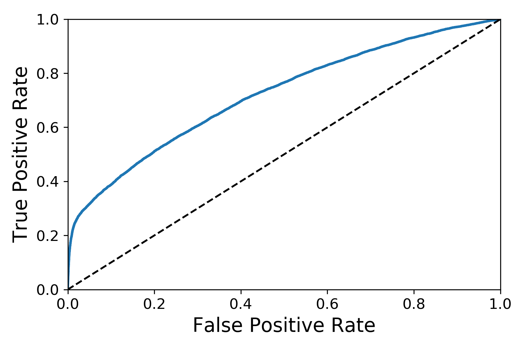
plots a ROC curve for the Logistics Regression classifier without tuning.
7. Model Tuning and Evaluations
Once Logistics Regression trains the model, I first evaluate the model’s performance. Next, I can use Scikit-Learn’s GridSearchCV to search the best hyperparameters for me.
The result is in figure 9.
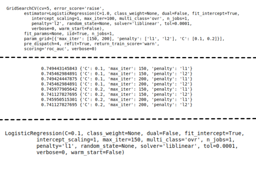
shows model tuning setup and result.
Furthermore, I need to also look for variable importance, i.e., which variables have proved to be significant in determining the target variable. The result is in figure 10.
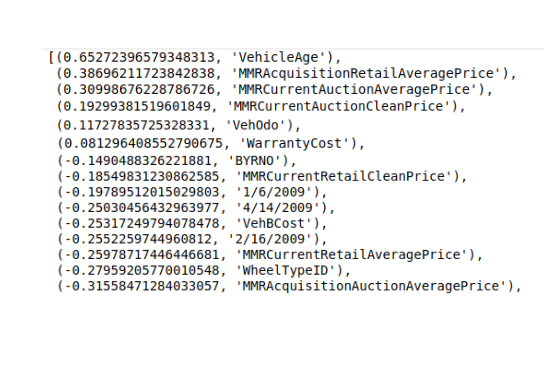
shows variables’ importance.
Moreover, accordingly, I can shortlist the best variables and train the model again. Finally, I use different algorithms to train the model. In figure 11, I plot three ROC curve for different algorithms: Logistic Regression, Random Forests, and Nonlinear SVM.
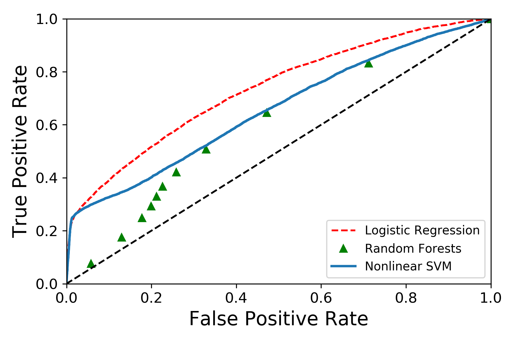
polts three ROC curve of different classifiers with tuning after modifying data features.
In the end, I will use those classifiers on test dataset to generate final classification.
The result is the figure 12.
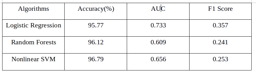
shows a table to compare result for three classifiers.
Reference
- Aurélien Géron. (2017). Hands-On Machine Learning with Scikit-Learn and TensorFlow. Sebastopol, CA: O’Reilly Media, Inc.
- Don’t Get Kicked! (2012) training & test [Data file]. Retrieved from https://www.kaggle.com/c/DontGetKicked/data
- Albert, H., Robert R, & Xin, A.W. (2012). Don’t Get Kicked - Machine Learning Predictions for Car Buying. Retrieved from http://cs229.stanford.edu/proj2012/HoRomanoWu-KickedCarPrediction.pdf